A presentation based on the concepts and ideas from this article was delivered at PyCon APAC Thailand in November 2021. Video of the presentation can be viewed on YouTube.
This is part 1 of a 2-part series. In Part 2, we will deploy a console-based simulator written in Kotlin, whose execution speed is about 10 times faster than this Python version.
Overview
Earlier this year, your author came up with some ideas that he hoped to assemble into a new viable alternative blackjack game. Creating a new blackjack game, or really any gambling game, is tricky because the game's mathematical House Advantage (the odds, or the amount of profit a casino can expect per unit bet) must fit in a rather small window. And among all table games, Blackjack typically has the lowest House Edge. A typical game with a 3:2 payout for natural Blackjacks will be around 0.55%1.
A successful new blackjack variant's House Advantage should be a bit higher than conventional blackjack, because casino managers will resist trying out a game with a lower edge than what they already have. But the new game's H/A cannot be too high or players will find themselves losing too much, too often. So although I had the bones of a new game in my head, I still needed to hone in on the exact set of rule adjustments and restrictions that would result in an ideal House Advantage. Further, blackjack involves player strategy and decision-making, so every proposed rule change also necessitates re-verifiying the ideal player strategy, while games like craps or roulette have no player strategy to consider at all.
The only way to do try lots of rule combinations, find the ideal player strategy, and measure the new House Advantage is to build a model and simulate millions of hands each time. Modeling a real-world Blackjack game, with multiple people at a table playing different strategies, is not terribly difficult, but it is more complex than it seems on first glance. Because of the reasonable possibility that a bug could sneak into my code (shocking!), I built two independent models in order to check my own work. One is a console application written in Kotlin and the other is a Jupyter notebook written in Python, which is what we'll discuss here. In both cases, being able to run more hands in less time was important to prevent slowing down the game development, and so I investigated ways to utilize concurrency, and how to take advantage of powerful cloud servers like the 16- and 32-core machines available to rent by the hour at Amazon EC2.
The Python model, wrapped in a Jupyter notebook, can be found on Github. You can download and run it yourself (v. 3.8+), or just follow along in the viewer. You can see the list of dependency imports in the first cell – if you are going to run it, be sure to pip install any packages you don't already have.

Of course by now, the game rules and payouts and optimal player strategies have been finalized, so we're just demonstrating speeding up the code. During development, however, I was constantly tweaking different aspects, running the simulation, evaluating the calculated results and refining the game further.
A super-detailed walkthorugh of the simulation's code is best suited for its own article, but we start by defining the deck of cards, and the payout values for every outcome. The next cell defines the player strategies for doubling down and splitting. Beyond that we create classes for each element – Card, Shoe, Hand, Player, Dealer, and finally, Game. Most are relatively straightforward, the Shoe class, for example, has a pitch() method for delivering a card to a Hand and a shuffle() method. The Hand class has a number of properties to check whether a hand is a natural, hittable, splittable, a "soft" hand, etc. The Player class has methods for making split, double and hit/stand decisions, referencing the player strategies we defined earlier, as well as properties for keeping track of money won and lost. The Game class coordinates the actions of the Dealer and the Shoe filled with Cards, and the Players, and it will determine the payout for every hand.
Running simulations
The first game simulation method we define is simple_loop(). In the next cell, we set the number of games to simulate at 500,000 and prepare the method call with a single player. We surround the method call with timer() calls to measure our speed, and as you can see from the output below, this loop takes about 51.8 seconds to run, approximately 9,650 bets per second. Nice, but we're going to need to do a lot better than that. In order to get a good estimate of the House Advantage that is accurate to within about 0.02%, we'll need to simulate at least 100 million hands.2
The next, most obvious change is to add more players to the game. Just like a real casino blackjack table, our simulator allows multiple people to play against the same dealer. When we run simple_loop() with 5 players, we only need to run 100,000 loops to simulate the same 500,000 games (of course, each loop takes longer), but we can get through it in about 35.5 seconds, just over 14,000 hands per second. Already, a 50% speedup.
Next, we will incorporate a library called joblib whose slogan is Embarrassingly parallel for loops. It's a perfect fit for our use case, which is running loops of the same game simulation hundreds of thousands of times. Python has a number of solutions for running asynchronous or parallel code, such as asyncio, multiprocessing and greenlet, but joblib requires very little refactoring, manages everything behind-the-scenes, and is easy to experiment with. We don't have to make any changes at all to our game code, but we do need to re-combine all the joblib results.
If we run 10 simultaneous jobs, our results from joblib will be a 10-element list. Since our goal is to calculate the win/loss for each of the 5 players, then combine those into an overall win/loss (from which, we'll caclulate the House Advantage), we have to combine the player results across the result list. In other words, if we have a 10-element result list, we need to combine "Aaron's" results across all 10, then "Bobby's", etc. Fortunately, the Counter class's update() method, sums identical properties across objects, which is the exact math calculation we'll need. These extra steps to re-combine the partial results from joblib are a bit tricky to get right at first, but they are the only code changes needed.
Our old kickoff was loop_results = single_loop(get_players(), bet_amounts, games_to_sim), which we replace with loop_results = Parallel(n_jobs=8)(delayed(single_loop)(get_players(), bet_amounts, games_per_loop, i) for i in range(loops)). The method call remains, we just have to add the number of jobs, and joblib takes it from there. Unlike the previous loops, where our mid-loop status updates (every 25,000 loops) are sent to Jupyter's output window, under joblib those results will appear in the console that launched Jupyter. My ancient computer, with just a 2-core processor, has limited ability to divide up the job, but still runs the half-million games in about 24.8 seconds, or about 21,100 hands per second, another 50% speedup. At this pace, we could complete about 75 million hands per hour. But in order to get a major speed boost, we're going to need something a whole lot more powerful than a single PC.
We're going to utilize AWS EC2 servers, which run the gamut from 1 to 64 cores, to really take advantage of parallelism, and turbocharge our game simulation. AWS bills by the minute, so the quicker we can complete the simulation, the less it will cost us. Even better, AWS offers huge discounts for "spot instances," unreserved servers currently sitting idle. These are poor choices for a production environment, because AWS can shut them down at any time to redirect to a reserved customer. But for short-term tasks like ours, they are a fantastic bargain.
(See the appendix below for creating your environment to run Jupyter notebooks. You need a properly-configured SSH client, and you need your AWS account to have a launch template with a prepared AMI disk image. For now, we're going to assume you have all of this already)
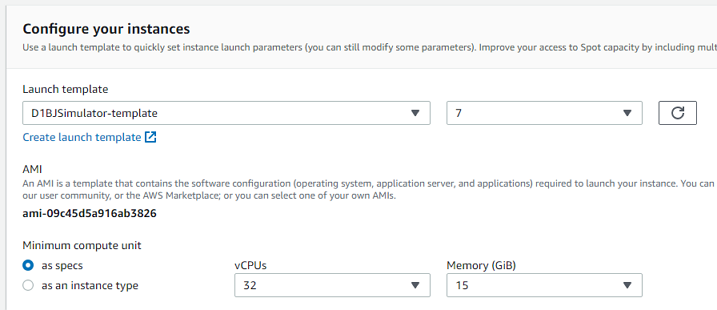
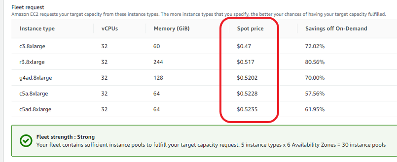
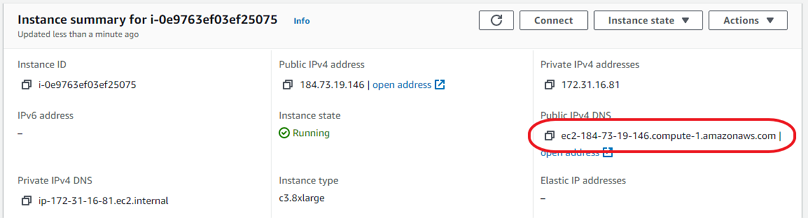
Log into the AWS console, go to EC2, then choose Spot Requests. Select your launch template, and set the minimum specs, 16 or more cores. Scroll down and we can see the possible instance types and the cost. 50 to 70% off is not unusual, especially at off-peak times, so not much more than 50 cents per hour. After a short wait, click Instances and you'll see that you now how a running instance (if not, you might have to wait another minute or two). Click the Instance ID to see the details. We're going to need the Public IPv4 DNS. Remember, every time you launch an instance, it's a new server with its own IP address. So every time, we will need to update the remote address in our SSH program. Keep in mind our instance is running, and we're being charged, so now is not a good time to be figuring things out for the first time.
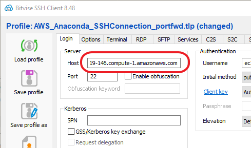
I really like the Bitvise SSH Client to connect to remote servers. It does a good job of key management, and provides both a console window and an GUI SFTP window for each active connection. Even if we have a saved connection template, we will need to paste in the new instance's DNS address:
After connecting, it is likely you will need to get the latest version of the notebook onto the server. Remember, the AMI disk image will only have files from the time it was created. If you've done any additional development, or made any changes at all, the server's version won't match the latest version. You can use a git pull, but since notebooks are self-contained single files, it might be easiest to simply open an SFTP window from Bitvise and drag the file from your local computer to the server.
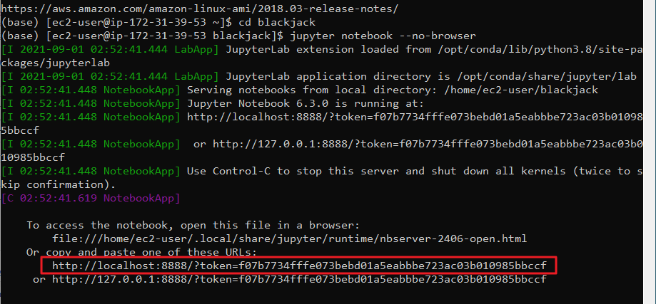
Next, open an SSH console, navigate to the folder with your notebook and launch a headless version of Jupyter: jupyter notebook --no-browser. When it starts, Jupyter will tell you its URL and token to connect. We want to copy that address from the console and paste it into our local browser, except we must change the port number to our forwarding port. So http://localhost:8888/?token=<token> becomes http://localhost:9999/?token=<token>. The interface is the browser on your local computer, but the code is actually running on your AWS instance.
Now, we're ready to go. You can play around with the number of simultaneous jobs for joblib, but I've found that a number equal to, or 2x the number of cores usually produces the fastest runtimes. So for a 32-core machine, either 32 or 64 jobs. We can run the notebook from the top, one thing to notice is that the non-parallel simple loops have barely any speed difference from our own computer, perhaps a few percent. But at the bottom, when we run in parallel thanks to joblib, that's where we see a massive reuction in time. Our 500,000 hands complete in under 3 seconds. 10 million hands only take about 41.6 seconds, and 250 million takes about 17 minutes. Now we're completing about 240,000 hands per second, more than a 10x speedup from the fastest run on our local computer.
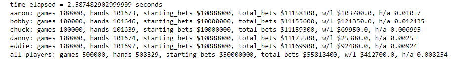
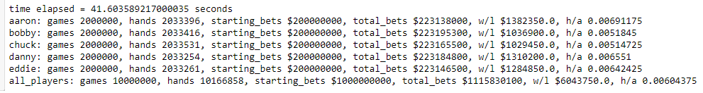
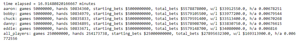
It's important to note the final value for House Advantage on each of the runs. After 500,000 hands, the H/A is calculated at 0.008254 or 0.825%. After 10 million hands, it was calculated at 0.604% and after 250 million hands, 0.677%. Of course, every run will be different, since the cards get shuffled randomly. What is important, is to run enough hands to eliminate volatility between runs, giving us confidence that our result will be replicated in future simulations, or by other models of the same game. Ss we stated earlier, our goal is to match the results of this Python model with our Kotlin model, which is able to simulate even more hands by nature of being compiled. After running billions of hands, the Kotlin model calculated a H/A of 0.67%. So the 250 million hand run matches! And it also demonstrates that even 10 million hands is not enough to produce a precise result. If we didn't have a second model, we could re-run this Python sim multiple times, gradually increasing the loop count until we get sufficiently consistent results every time.
Make sure to go back to the AWS console and terminate your instance! Doing so will ensure your costs are capped at under a dollar. Forgetting to do so will continue to accrue charges, possibly for days or weeks! However keep in mind that none of your work will persist once you shut down the server. If you've made significant changes to the notebook, don't just save it (which will save it to the server's filesystem, which will get wiped), but use the Download As... option in the File menu to save it to your local computer, probably as a Notebook (.ipynb) but possibly a Python script (.py).
Oh, and about that blackjack game... it's now a real game called Cheat At Blackjack®! You can even play it online right now!
Appendix: Preparing your environment for the first time
The most important thing you need to do is to have an AMI disk image that is capable of running your code. In this case, it's Python, Jupyter and the specific packages our notebook expects to import. If you also want to run a Kotlin console application, you'll need a Java JVM. You do need to run a live instance in order to build an AMI, however, you can do so on very low-level types that just cost a penny or two per hour. Later, you'll be able to use the saved AMI on a much more powerful server.
You can completely start from scratch and build the disk image off of a raw Linux distro, or find an existing AMI that already has some of the pieces installed from the AWS Marketplace. The latest Anaconda images already have Python installed, Jupyter installed, and importantly, they are free to run (other AMIs charge a usage fee on top of the cost of the server), so they are an excellent choice, even if you don't use Anaconda day-to-day.
Log into AWS, go to EC2, click Instances then Launch Instances. On the next page, search for Anaconda and find the latest version in the Marketplace (pick the x64 architecture), or your favorite Linux distro if you'd prefer to build from scratch. Pick a very basic Instance Type such as t2.medium. If this is your first-ever time launching an EC2 instance, you may need to set up a VPC, Subnet and/or Security Group – please refer to Amazon's own documentation for how to do that. You can skip adding Storage. However when you click Launch, you will be asked to create a key pair. Name it, then download it. As AWS will tell you, you cannot re-download the key file again, so be sure to save the one you've got in a location you'll remember.
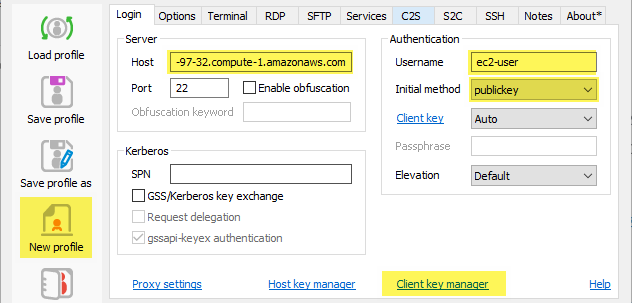
AFter a few seconds, your new instance will be up and running. The next step is to connect to it over SSH. If you're familiar with PuTTY, go ahead and use that, however, I believe the Bitvise client is much simpler, if you're running Windows, and it allows configuring port forwarding in a profile, which we will need. In Bitvise, create a new profile. First thing, go to Client Key Manager, click Import, change the file type from .BKP to any, and import the .PEM file you just downloaded (note how you didn't have to convert to a PuTTY .PPK file). You can add a comment such as "aws-ec2-key" to make it easier to recognize. Back in the profile, copy the instance's Public DNS to Bitvise's Host field, Port 22, Username "ec2-user", Initial Method "publickey". You can specify the key you just saved or leave the key selection to Auto.
Now click the C2S tab to set up port forwarding. Click Add, listen on 127.0.0.1, port 9999 (or any port you choose), and set Destination Host to "localhost", port 8888 (don't change this one). This is necessary to run Jupyter on a local browser and connect to the remote server's Jupyter engine.

At this point, attempt to connect. You should not require a password, as the key will automatically allow you to login. Check your Python installation with python --version. Same with jupyter: jupyter --version. Java only requires one dash: java -version. You can check all the other Python packages with pip list. You should probably update all system packages with sudo yum update followed by sudo yum upgrade (some systems will use apt-get rather than yum). Anything else you might want to install, or secure, or configure on a new Linux box, you can do now. Return to your home directory with cd ~ and create a project directory: mkdir myproject.
In Bitvise, open an SFTP window, navigate to the new project directory you just created, and if there are any files you want to copy, you can drag them in. You can also use the console to git pull any repos. It may be preferable NOT to upload your actual notebook or project files, because we're going to freeze this filesystem, meanwhile, it is likely you will continue to develop your code, and you'll only want the newest version.
Now, return to the AWS EC2 dashboard, go back to Instances, select the active instance, and choose Actions > Image and Templates > Create image. Provide a name and save. Go to Launch Templates, click Create Launch Template, provide a name, and in AMI selection, search for the name you just gave to the AMI image. You don't need to specify an instance type but you should include the key pair – this will ensure that the key you saved will continue to work on all future instances from this template.
Go back to Instances and terminate the one you initially created. Go to Launch Templates and click Actions > Launch instance from template. Select an instance type and Launch. Alternatively, you can go to Spot Requests, click Request Spot Instances, select your Launch Template (which should automatically select your AMI), and pick the minimum specs or type. Again, we're still in setup mode, so pick a minimal type, launch it, wait for the instance to start, then follow the instructions in the main article to get your notebook on the filesystem, start Jupyter, and connect.
Again, make sure you terminate all your running instances!
Footnotes
-
The House Advantage calculation is simple: Total Win / Total Initial Bets. The "Win" is calculated from the casino's side, so it's equivalent to Player Losses. Unlike most other games against the house, blackjack allows players to increase their initial bet, by doubling down or splitting. This leads to an alternative measure, Element of Risk, which is Total Win / Total Bets, although most casino managers, regulators, and analysts will focus on the House Advantage. ↩
-
Some games can be "solved" empirically, that is, purely with math, without simulating the game. For example, Roulette has exactly 38 spots (1-36, 0, 00) on the wheel. A bet on a single number pays 35-to-1. Therefore the total payout matrix is (1/38 * 36) + (37/38 * 0), or 0.9474, that is, for every 1 unit bet, the house can expect to pay 0.9474 unit, and keep 0.0526, for a House Advantage of 5.26%. It's the same for betting on Red or Black, or Even or Odd, all of which pay even money: (18/38 * 2) + (20/38 * 0) = .09474. Dice, where there are only 36 possible outcomes (62), can also be solved. But card games, where the size of the hand is variable, and where players make decisions, and the hands compete against each other, are better suited for simulation. ↩