The April 2017 issue of Global Gaming Business magazine includes an “exploratory study” which claims to reject the hypothesis that gamblers can perceive differences in slot machine hold percentages. The study was authored by two university professors, providing the appearance that this was a valid, well-researched, evidence-based trial overseen by experts. In fact, this study was flawed, possibly fraudulently, in nearly every way, including the initial hypothesis, the experiment’s design, and the interpretation of the results.
First, the reasoning behind the experiment is unclear, contradictory, and plain wrong.
We performed a study to empirically examine how changes in PARs affect game performance at a tribal casino.
[Author’s note: for explanation of PAR, hold percentage, payback percentage, theoretical hold & win, please see appendix below the article]
Except that as we will see, the PARs (the theoretical hold set by the game’s internal configuration) never changed throughout the experiment. One might be interested in how a single machine, after being set at, say, 9% hold for a year, performed before and after adjusting the hold to 11%. But that is not what this experiment measured.
In particular, we created an experiment to determine whether slot players at this property can, in fact, detect considerable differences in theoretical payback percentages.
This is a classic straw man argument. Nobody claims that players can detect a game’s theoretical payback (or differences between two games’ paybacks) in isolation, only that players can potentially detect differences in actual payback percentages. Normally, over time, theo and actual line up. However, if during the experiment, they diverge instead of converge, the observers must acknowledge that the gamblers in the study could not be expected to respond to a theoretical payback percentage that was not realized, any more than people would not respond to a “theoretical” sunny summer day when in reality, it is raining and windy outside. (Foreshadowing the results, this will become important.)
The long-held idea that changes in hold percentages can be detected by players has been cited by some organizations and individuals as the cause of declining slot win in U.S. casinos, most of which cater to a local repeat clientele. If this assumption is true, then the tribal casino operator we worked with should expect to earn less on slot machines that offer higher holds, provided their savvy players have a sufficient amount of time to detect the relative “tightness” of the machines.
This assumption distorts the relationship between a product’s price and its popularity and profitability. Slots are unique in that the “price” of a slot machine, its house advantage, is unknown by the player (the degree to which experienced players can deduce the price is, supposedly, what is being tested). But even where pricing is transparent, such as with 6/5 blackjack vs. traditional 3/2, a less popular game can still earn more for the house, if the higher odds outweigh the demand elasticity. Thus, “should expect to earn less on slot machines that offer higher holds” is another straw man argument, providing cover to shift the experiment from directly measuring player demand to measuring casino profitability. Again, nobody doubts that if holds are sufficiently low, raising them slightly can result in higher profits, even when players can perceive the difference.
All game pairings [authors note: 2 pairings in total] comprised two identical games, save the difference in theoretical percentages. The paired games featured the same visible pay table, the same theme/title, the same credit value (i.e., $0.01) and the same cabinet design.
What was studied, was not reaction to changes in theoretical holds, but the performance difference between two games which appeared identical to the players. Identical, except for this tidbit:
This tribal gaming facility located one game of its two-game pairings on the lateral end of a bank, with the second game located directly adjacent to the first game (i.e., a side-by-side configuration). The second game occupied an interior/middle-unit position within the bank.
Flaw #1: Not eliminating, or controlling for, a major, external bias. Supermarkets have end-caps, magazines have back covers, retail has traffic intersections, and casinos have end-of-row locations. High-traffic, high-visibility locations have a built-in advantage and cannot be fairly compared with identical units that don’t share the same location advantage. Yet, this study sets out to compare an end-unit placement with an interior unit, without attempting to measure the size of the bias, or indexing the results to mitigate its effect. The authors acknowledge the location advantage, but completely underplay the influence: “researchers have found end units to be associated with increased game performance.” Not just researchers, but any casual observer of a casino floor can quickly surmise that end units tend to have a location advantage. Further, despite acknowledging it up front, the authors completely ignore the bias when discussing the data, interpreting the results, and publishing a conclusion. Yet this large bias infects the entire experiment and unquestionably invalidates the conclusions eventually stated by the professors.
Flaw #2: No discussion of preconceived player bias. Another possible source of bias is the players previous experience with the game themes and machine location used during the test. The test began on May 1, so experience with the themes or locations in April, March, or earlier could easily have influenced some players during the test period. Unfortunately, we know nothing about the prior history of these themes and locations. Did these specific themes, Chilli Chilli Fire and Mystical Ruins, exist in the test location, or elsewhere on the gaming floor, prior to May 1? Prior to the test’s start, would some players have been exposed to the test themes, configured with higher hold percentages (“tighter”)? During the test, were other machines with these themes available elsewhere, set at higher holds? The authors did nothing to counter or even review this potential source of bias.
Flaw #3: The test variables are not realistic. The hold percentages being tested, 5.91% and 8.01%, are significantly lower than typical penny game configurations. Even the high-hold game, at 8%, is a bargain compared to typical penny machines configured to hold 11%, 13% or even 15%+ in some cases. (In New Jersey during 2016, for example, 1- and 2-cent games held 11.2%, while every other denomination held between 6.1% and 9.0%. source: NJ Dept Gaming Enforcement). Since even the 8% game was likely much looser than the majority of penny machines at the casino, a player who could perceive slot hold differences would notice the huge reduction in hold between this game and the majority of other units, and therefore be likely to stay loyal to that particular machine.
Flaw #4: Testing one segment of demand curve, then claiming conclusions over entire curve. As mentioned, the experiment only looked at differences in player behavior between 5.9% and 8% holds, despite the fact that most floor averages are higher, and penny games, as a whole, are usually much higher. Yet the authors believed that these limited observations would apply universally to any level of hold percentages — that the experiment’s conclusions would also be valid when comparing, say, 11.9% to 14%. This is a misguided assumption to make in any case, but even more so when the test is so far away from the practical application to penny games which are well into double-digit holds.
Flaw #5: Incorrectly assuming hold differences in high-volatility titles are equally noticeable as low-volatility titles. Whether or not the professors were aware ahead of time that Mystical Ruins’s pay table is more volatile than Chilli Chilli Fire’s, the standard deviation of the daily actual wins ($466/$502 vs. $677/$931) makes that fact clear. But the study makes no allowances to provide customers additional time to perceive the hold difference in the more volatile game. Perhaps the following thought experiment will clarify:
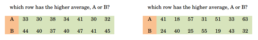
Because the rows in the left test are much less volatile, it takes far less time to determine whether A or B has the higher average. The left test can be answered almost immediately, while the right test requires a bit more time, even though, in both tests, the difference in the averages is identical. Similarly, players on high-volatility machines will get a wider range of feedback (spin payouts), and therefore, it takes longer to accurately assess high-volatility games. However, the experiment not grant additional time, it did not grant any “feeling-out” time at all…
Flaw #6: The test allows no time for player discovery and experience-building. Related to the previous point, players need time and experience to form an opinion of a game. Even the professors recognize that that behavior differences would only arise after “savvy players have a sufficient amount of time to detect the relative “tightness” of the machines.” However, the test setup does not allow for any assessment time, as they begin gathering result data on Day 1 of the test. A useful study would have ignored result data for the first 2 to 3 months after installing the games, giving players sufficient time to try them out and begin forming an opinion. An even better study would compared the differences in the relevant statistics across time. In other words, if Game A outperformed by 20% in month 1 (due to the location bias), before players could have detected a difference, how much did it outperform during month 6? I.e., as they gained more experience with the test games, did players shift more game play towards the looser game?
Flaw #7: Result data includes players who are not qualified. Again, nobody claims players could perceive hold percentage differences* without a good amount of experience playing both games*. But the result set includes all players at all times, regardless of whether or not they are in a position to notice a difference. Specifically, the test makes no attempt to exclude results from players who only played one of the games in a pair, who, by definition, are unqualified to determine which game might have a lower hold percentage. They also fail to exclude results from players’ initial sessions with the games, before which, they could not possibly have been able to tell a difference. A better test would have filtered results to include only specific players (which is possible via player card tracking) who played both games in a pair and registered some minimum amount of hours on each.
Flaw #8: Factually incorrect result summary. Reviewing Table 2, it is easy to see that the 8% game, the one at the end of the row, tallied a higher coin-in total (amount wagered), as measured by both mean and median, on both pairs of machines. Yet the authors write:
The mean coin-in was greater for the games with the least PAR in both pairings.
This is simply wrong, according to Table 2. And if it was correct, it would be in total opposition to the authors’ eventual conclusion.
Flaw #9: Relying on un-transformed data for t-test analysis, despite slot outcomes not being normally-distributed. Table 2 shows that the maximum daily results for coin-in and theoretical win are consistently much further from the mean than the minimums. For example, the first row shows a mean of $232 theoretical win, with a sigma of $103. The minimum value is $65, or 1.6 sigmas away. But the maximum value is $814, or 5.6 sigmas. The other theoretical win calculations all follow. The authors could have used a log transformation, reciprocal square root, or other methodology, to attempt to normalize the data before subjecting it to t-test analysis, which expects a normally-distributed population.
Flaw #10 — the most egregious error of all: Experiment ignores the failure of the tested variables to perform as anticipated, invalidating the premise entirely. Unfortunately for the study, the games themselves did not play “true.” Both 5.9% theoretical games actually held over 7%, while one of the 8% games actually held just 4.35%, making it far looser than any of the other 3 games in the study. Normally, over the course of 6 months — hundreds of thousands of individual spins — games pay out close to their theoretical configuration (PAR, in the authors’ terminology). But unfortunately for the study, that did not happen, which totally invalidates the study’s results. Player behavior can only be measured according the feedback they actually experience — and during the study, one game held just 4.4% while its counterpart paid 7.3%. The fact that the game results should have been inverted, based on their PAR configurations, is totally irrelevant because it simply did not match up with reality. (And for the other pair, instead of a 2.1% absolute difference in hold, the actual difference was just 0.65%, which any rational observer would acknowledge is far more difficult for individual gamblers to perceive).
While the fact that the games did not deliver the expected results is not the fault of the professors, their decision to ignore it and to publish their results, as if the actual game results had no impact on player behavior, is irresponsible and demonstrates personal bias. If a scientist wanted to study the effects of drought conditions in California, running a study during the record rainfall of 2016/7 would unfortunately, invalidate the data. The base variable that was at the core of the test — the different hold percentages among the individual machines — became “corrupted” by real life and did not stay true to the experiment setup. Not just a small amount — the “high-hold” game was actually much looser than its counterpart. Not the professors’ fault, but a fatal flaw nonetheless. They have a professional responsibility not to publish misleading results.
Despite all of the experiment’s flaws, and the huge bias baked into its design, the authors still could not achieve the clear, convincing outcome they were seeking. They still needed to be quite creative and compensatory to reach the conclusion they sought, which they did by using a very generous 0.10 alpha-value against which to assess statistical significance, ignoring statistical measures that were unable to achieve significance, instead of acknowledging them, and by failing to consider alternative explanations of the result data.
Flaw #11: Failure to consider alternative interpretations of the results. If the professors weren’t going to throw out the experiment due to #10, at least they could have looked at the result data in a bit more detail, and from a different perspective. They knew up-front there was a bias due to location, so instead of ignoring this bias, they could have utilized it. The results below are calculated solely from the original article’s Table 2. It shows that with Chilli Chilli Fire, where the two units’ actual hold percentage was very close (8.25% to 7.60%), the end row location advantage was worth an 18% premium in coin-in. But with Mystical Ruins, where the end game was much more advantageous to the players (4.35% to 7.26%), the end row advantage grew to a 30% premium in coin-in. In other words, when the gap in hold percentage widened, players DID respond by playing the looser game much more. The mean coin-in gap widened from $715 to $1,109 per day between pairs, as players placed 57% of their Mystical Ruins wagers on the game with the end location and lower hold, compared with 54% of Chilli Chilli Fire for the end location without the hold advantage. In direct opposition to the published results, customers increasingly selected the low-hold game. If we could isolate just months 4–6, it is highly likely the contrast would be larger.
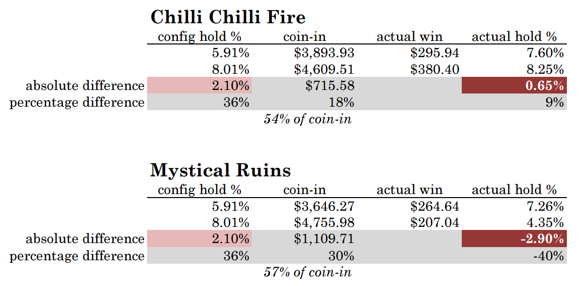
To repeat: the study showed that when the gap in actual, observed hold percentages widened between the games in a pair, players directed more of their play to the looser game. This directly contradicts the authors’ stated conclusions.
Flaw #12: Because the initial hypothesis was flawed, the authors chose an irrelevant statistic upon which to base their results. As noted earlier, “whether slot players at this property can, in fact, detect considerable differences in theoretical payback percentages” is a straw man argument. But since this flawed assumption revolved around theoretical win, the authors chose to measure theoretical win, instead of a more direct measure of player preference, such as coin-in, handle pulls, total time on device, average session length, likelihood of a second (or third) session, share of wallet, average time until abandonment, or other possibilities. However, theoretical win alone is simply not a good measure of customer behavior, as its entire purpose is to eliminate the influence of “luck,” which may be a useful exercise for executives but is completely dismissive of the player experience and reason for gamblers to visit the casino in the first place. Further, it is purposely confusing for the researchers to focus on this statistic, because it measures what should have happened, as opposed to what did happen, which conflicts with reality when actual results do not match theoretical results, as we already discussed in #10. It would be like proclaiming Atlanta Falcons fans are irrational for expressing disappointment after Super Bowl 51 because, theoretically, with their large lead, they should have won the game, instead of observing what actually occurred.
Flaw #13: Selectively ignoring statistically-sound results that contradict the desired outcome. The authors provide data for 3 measurements, for illustrative purposes, but choose to base all their conclusions on just one:
Two-tailed, two-independent-sample t-tests were conducted using the daily theoretical win for each game shown in Table 1. … hypothesis tests were not conducted on daily coin-in and win observations
But with the data in Table 2, we can calculate t-test values for all 3 statistics, and we find that Actual Win failed to reject the null hypothesis. No wonder the professors didn’t use it!
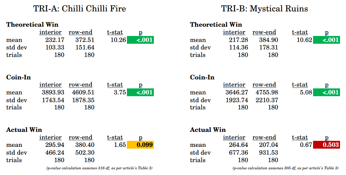
Surely the professors did the same calculations, then chose to ignore the results that did not agree with their desired outcome, and re-focused the story only around theoretical win instead.
The results did not support the notion that players could detect the differences in the PARs over extended periods of time (e.g., 180 days). The findings did support a strategy of increasing the theoretical hold percentages to improve game performance. Such results could be valuable to operators seeking to improve slot revenues, as gains may be possible via increased theoretical hold percentages.
In summarizing their conclusion, the professors conveniently ignore the large inherent bias in the games’ locations, and further, ignore the measurements (Actual Win) that contradict the desired outcome. Where, exactly, this lies on the spectrum of ignorance, incompetence, and/or fraud, is left up to the reader to decide.
Global Gaming Business is a respected industry magazine, but unfortunately, publishing this article represents a hit to its credibility. This study suffers from multiple major flaws in design, had an initial premise that was inaccurate and misleading, and reaches conclusions which are not supported by the data. There should have been more review and criticism of this study before going to press.
Appendix — explanation of casino and slot machine terminology
A slot machine’s payback percentage is the amount of wagers it returns to players as wins. In other words, if, over the course of a day, a machine accepts $1000 worth of wagers, and pays out $900 in wins, its payback percentage is 90%. The compliment of this is hold — the amount won, or “held” — by the house. In our example, the machine held 10%. Payback percentage + hold percentage will always equal 1.
“Coin-in” (sometimes called “handle”) is simply the total amount of wagers — $1000 in the example above.
“Penny games” are slot machines with a 1-cent denomination, which currently make up the vast majority of “video reel” (i.e. virtual) slots. Despite the 1-cent denomination, games cannot be played for 1 cent per spin, or anything close. Most offer 30, 40 or more mandatory “win lines,” plus “multipliers” ranging from 2x to 10x or more, so that individual spins on penny machines usually range from 40 cents to three or five dollars.
The theoretical hold percentage, colloquially called “theo” (synonymous with PAR, the professors’ preferred terminology, as well as theoretical win percentage), is the machine’s expected hold percentage, based on its internal configuration. However, there is no guarantee that actual game results will match the theoretical configuration, just as there is no guarantee that if you flip a coin 10 times, you’ll get exactly 5 heads. The more individual trials, the more likely that collective game results will eventually reflect the theo, but an individual machine can diverge from theo for reasonably long stretches. According to the data in this 180-day experiment, one of the Mystical Ruins games was configured to hold 8.01%, but actually won only $207.04 per day from $4755.98 in daily wagers, or 4.35%. The 3 other observed games’ actual hold percentages were all much closer to their theoreticals.
The “theoretical win” is a measure casino executives use that allows them to measure performance after removing the variability of luck. The theoretical win is simply actual wagers x theoretical hold percentage. So for the Mystical Ruins game which collected $4755.98 in wagers (coin-in) per day, the theoretical win is 8.01% of that, or $380.95, because 8.01% was the theoretical hold percentage. But as we just saw, the actual win was less, just $207.04 per day, over 180 days. The reason that theo win is a poor choice for measuring customer behavior is that, by definition, it always assumes every game outcome matches the expected value, when in reality, players experience a wide range of outcomes — big jackpot wins, stretches of losses, sporadic mid-sized wins, near-misses, etc. — that greatly influence a player’s perception of a game as well as that player’s future behavior (whether to continue playing, when to stop, whether to play again on the next visit, etc). Relying on theo in an experiment to measure player experience is like studying the atmosphere and ignoring daily changes and volatility in weather, substituting actual recorded temperature, precipitation and humidity during the study with their long-term historical averages and assuming zero volatility.